mechanical-engineering-skills
Tutorial: MeltpoolNet (process parameters → melt-pool size and mode)
Skill: meltpool-geometry · Paper: P. Akbari, F. Ogoke, N.-Y. Kao, K. Meidani, C.-Y. Yeh, W. Lee, A. Barati Farimani, MeltpoolNet: Melt pool characteristic prediction in Metal Additive Manufacturing using machine learning, Additive Manufacturing 55 (2022) 102817, doi:10.1016/j.addma.2022.102817 · Data: BaratiLab/MeltpoolNet
MeltpoolNet collected melt-pool measurements from more than 80 metal AM papers: power, speed, beam size, alloy, and the resulting depth, width, length and melt-pool mode. It benchmarks ML models with physics-aware features and fits explicit power laws that respect dimensional analysis.
This skill gives you three estimators, from most interpretable to most data-driven:
- Rosenthal
- a fitted power law
- ML models
It also tests honestly how well the ML models transfer to a machine they have never seen.
Use cases
- Planning single tracks: expected depth and width before a DOE, and whether W/D is heading toward keyhole mode.
- Choosing hatch and layer: melt-pool width and depth feed the overlap criteria in
lpbf-defect-prediction. - Teaching: Rosenthal scaling against measured data, absorptivity models, dimensional analysis.
- Adapting to your machine: measure a handful of tracks, add them with
--extra, and the model re-centres on your process.
Setup
npx skills add BaratiLab/mechanical-engineering-skills --skill meltpool-geometry
pip install numpy pandas scipy scikit-learn matplotlib joblib
cd skills/meltpool-geometry
1. Physics first: Rosenthal
python scripts/meltpool.py rosenthal --material SS316L --power 200 --velocity 800
The result is depth 59 µm, width 118 µm and length 462 µm, with absorbed power 66 W (minimum absorptivity 0.33 from the data). Rosenthal assumes conduction mode, so it under-predicts keyhole depths.
2. An explicit formula from data
python scripts/meltpool.py identify --target depth
The fit is y = w0·P^a·V^b·ρ^c·Cp^d·k^e·(Tm−T0)^f with the four dimensional constraints (mass, length, time, temperature) solved exactly; the residuals print as zeros. Result on 1,340 depth measurements:
| Exponent | P | V | ρ | Cp | k | ΔT |
|---|---|---|---|---|---|---|
| Fitted | 0.51 | −0.22 | −0.49 | −0.63 | −0.02 | −0.64 |
The P exponent sits right at Rosenthal’s ½.
| Target | Fitted power law R² | Rosenthal R², same rows |
|---|---|---|
| depth | 0.24 | strongly negative |
| width | 0.64 | strongly negative |
| length | 0.57 | strongly negative |
The paper reported 0.787, 0.991 and 0.473 for the power law. Its published equations don’t reproduce on today’s public CSV under any unit convention we tried. Report what you reproduce.
3. ML, and the question that matters: will it transfer?
python scripts/meltpool.py benchmark --target depth --features baseline,energy --split random --models gb --plot a.png
python scripts/meltpool.py benchmark --target depth --features baseline,energy --split paper  --models gb
python scripts/meltpool.py benchmark --target depth --features baseline,energy --split paper  --models gb --calibrate 10
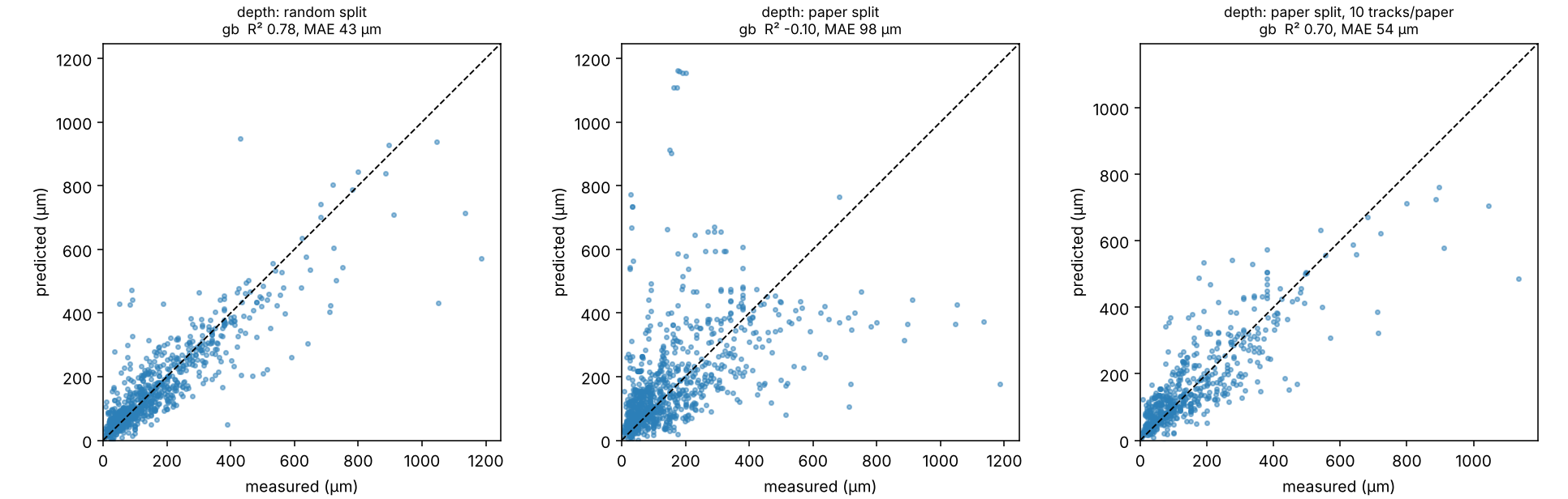
| Split | Depth R² | MAE |
|---|---|---|
| Random 5-fold, as in the paper | 0.78 | 43 µm |
| Leave-paper-out (whole source studies held out) | −0.10 | 98 µm |
| Leave-paper-out + 3 of your own tracks per study | 0.52 | 71 µm |
| Leave-paper-out + 10 of your own tracks per study | 0.70 | 54 µm |
A random split shares machines, powders and measurement methods between train and test. A new
machine looks like an unseen paper. The fix is cheap: measure a few single tracks and retrain
with --extra.
Melt-pool mode classification follows the same pattern: 82.6% accuracy with a random split (the paper reports 85.8%) and about 45% leave-paper-out.
4. Predict, with the caveats attached
python scripts/meltpool.py train --target depth --features baseline,energy --model gb --out depth.joblib [--extra my_tracks.csv]
python scripts/meltpool.py train --target width --features baseline,energy --model gb --out width.joblib
python scripts/meltpool.py predict --models depth.joblib,width.joblib --material Ti-6Al-4V --power 250 --velocity 1000 --beam 80
For Ti-6Al-4V at 250 W and 1000 mm/s, the output is:
- depth 132 µm, width 151 µm, so W/D = 1.15, which flags keyhole risk;
- Rosenthal: depth 61 µm, width 122 µm;
- the model’s leave-paper-out validation, attached so nobody mistakes the number for a measurement.
Notes
abs2(paper Eq. 3) is computed from the measured width, so using it to predict geometry leaks the answer. The skill warns when you request it.- The data is mostly SLM, with a little EBM, at 293 K ambient. Treat other processes and preheats as extrapolation.
Cite: Akbari et al., Addit. Manuf. 55 (2022) 102817.